How to produce a stacked plot of radiocarbon date density probabilities

Since introduced by the middle of 20th century, radiocarbon dating has been used in a large variety of disciplines. In palaeoecology, it has allowed for a major improvement in dating past phenomena. The ground principle is fairly simple: the isotope 14 of carbon (14C) is radioactive and decays following one criterion, namely the half-life. The half-life means the time necessary for the original quantity to reduce to half. For 14C, it is about 5730 years!

Living organisms, just like you, accumulate carbon in their tissues all life long. This includes a certain proportion of radioactive carbon as well, but don’t be afraid, you don’t bare any risk 🙂 This proportion is kept similar to the atmospheric level of radioactive carbon, but by the death of an organism, it is not renewed anymore and starts to decay. Half of it, every 5730 years. Therefore, if you can measure how much of radiocarbon is left in a sample today and how much of non-radioactive carbon it contains, you can use its half-life, do the reverse maths and deduce the date of this (sad) event.

However, the proportion of radioactive carbon against non-radioactive carbon is not constant. It has actually frankly oscillated during the last dozen of thousand years. This is why the result of your above maths need to be corrected. You can achieve this with a calibration curve. You will get a probable time span in calendar years, but some years are more likely than others. This is the density probability.

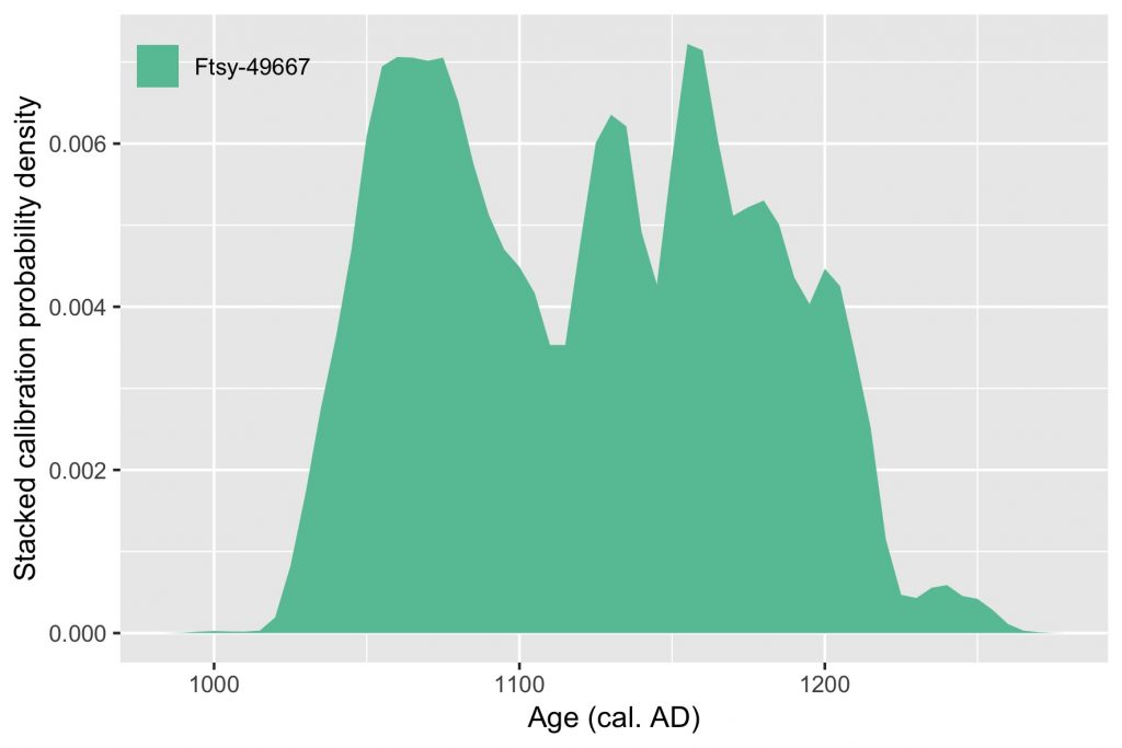
Nowadays, radiocarbon dating is rather cheap and fast, and scientists use them intensively. For instance, archaeologists find thousands of remains and radiocarbon dating ten or 100 or them can help figure out which period they come from. But unfortunately they won’t give the exact same result. An interesting approach to help making a decision is to pay attention to all these probabilities from the calibration of each date. All you need is love, of course, and R.

First, the packages. Always.

library(tidyverse)
library(clam)

tidyverse is used to handle data, and the function calibrate() from the package clam is used to… Well, to calibrate the dates.

Then, I generate some fantasists radiocarbon date results from the Middle-Age, but of course here you can use your own results.

(dates <- tibble(
  id = replicate(7, str_c("Ftsy-", str_c(sample(0:9, 5, replace = TRUE), collapse = ""), collapse = "")),
  c14_age = sample(seq(800, 1100, 10), 7),
  c14_error = sample(seq(20, 50, 5), 7)
))

See how an extra pair of parentheses both creates and displays the object dates at the same time.

Next is to create a function that will calibrate a date, using the values it finds in the data frame you provide to it.

bunch_calibrate <- function(x){
  id <- x %>% pull(id)
  cage <- x %>% pull(c14_age)
  error <- x %>% pull(c14_error)
  calibrate(cage, error, storedat = TRUE, graph = FALSE)
  dat$calib %>% 
    as_tibble() %>% 
    select(age = V1, density = V2) %>% 
    mutate(id = id)
}

Once you have it, you’re all set to do the fancy calibrations all at once!

(output <- dates %>% 
    split(dates$id) %>% 
    lapply(bunch_calibrate) %>% 
    bind_rows())

Here it is a bit tricky so let’s break it down. split() will create a list of data frames according to the values found in the variable id. Then, our previous function bunch_calibrate() is applied piecewise to each single date (since each date is now a single-line data frame in the list created with split()). And finally, the results of each call to bunch_calibrate() are bind together with bind_rows().

Note that the package purrr could make it easier to implement the split-apply-combine strategy here, but I haven’t learnt about this package yet 🙂

To go even fancier (I know, you wouldn’t have expect, right?), we order the dates by their weighted calibrated age :sunglasses:

(date_order <- output %>% 
  group_by(id) %>% 
  summarise(wght_age = weighted.mean(age, density)) %>% 
  mutate(id = fct_reorder(id, wght_age)) %>% 
  arrange(id) %>%
  pull(id))

final_output <- output %>% 
  mutate(id = parse_factor(id, levels = date_order))

Finally, last thing to do is a nice wonderful plot:

ggplot(final_output, aes(1950 - age, density, fill = id)) +
  geom_area(position = "stack") +
  theme(legend.position = c(0, 1), legend.justification = c(0, 1), legend.background = element_blank(), legend.key = element_blank()) +
  scale_fill_brewer(palette = "Set2") +
  labs(x = "Age (cal. AD)", y = "Stacked calibration probability density curves", fill = NULL)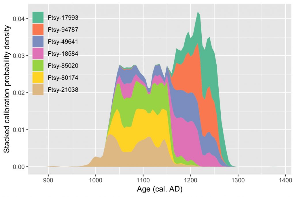

Isn’t it beauty?